
Detect Serendipitous Stellar Occultations with Deep Learning
Abstract
Introduction
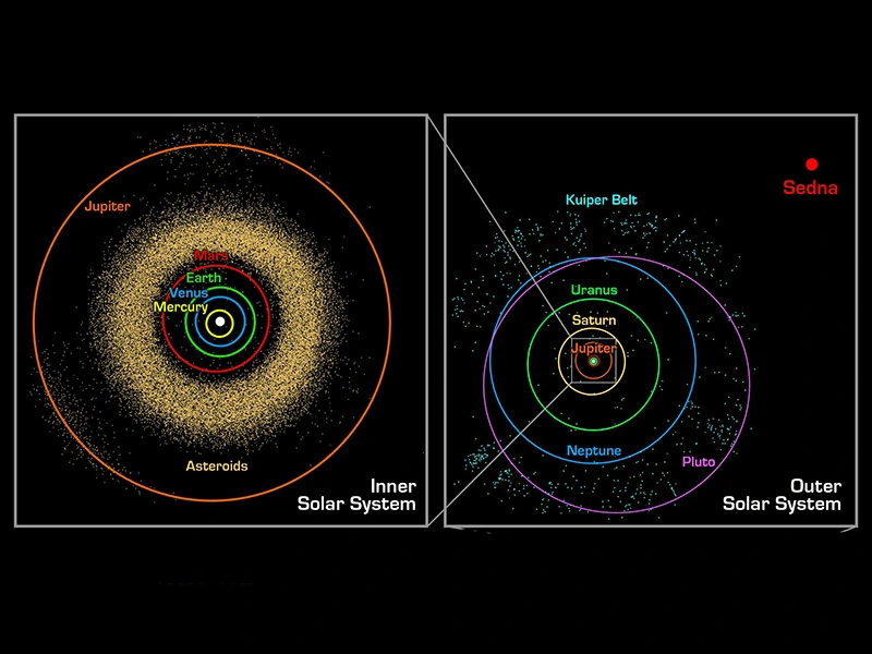
The TAOS-2 project is an international collaboration between Taiwan, the United States, and Mexico, focused on the field of astronomy. The primary aim is to conduct a comprehensive survey of objects in our solar system beyond Neptune, with particular attention to the Kuiper Belt, the origin of the majority of short-period comets. The project's findings are expected to shed light on the formation and evolution of our solar system and help refine current theoretical models.
The purpose of this pipeline is to detect small objects (such as comets and asteroids) in the solar system and classify them using GAN. These objects are detected through serendipitous (unplanned or unexpected) stellar occultations. An occultation occurs when one object passes in front of another from an observer's perspective. In this case, a small object passes in front of a star, temporarily blocking its light. Therefore, this problem can be reduced to finding an event in a time series.
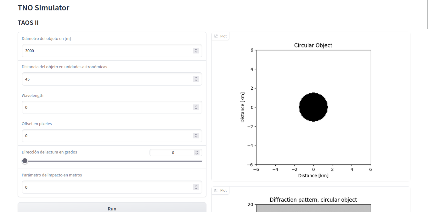
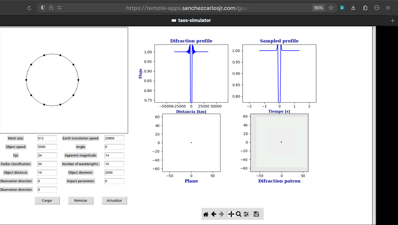
The pipeline analyses the light curves, which are graphs that show the brightness of an object over time. These light curves are the primary data source and they were obtained from the Trans-Neptunian Automated Occultation Survey (TAOS II) event simulator.
Various parameters affect the shape and properties of the occultation light curves, and these were explored in the study. Some of the parameters mentioned include spectral type, apparent magnitude, finite angular size of the star, angle from opposition, and readout cadence for the observations. Additionally, Poisson noise distribution was assumed in the data, as expected from the TAOS II project.
The classification is based on characteristics such as the size of the objects (which can range from a fraction to a few kilometers) and their distance from the Sun (typically a few tens of astronomical units). The objects of interest here are primarily trans-Neptunian, meaning they are located in the outermost region of the solar system, more precisely, in Kuiper belt and Oort cloud.

Related work
Different ways have been proposed to detect and classify a lightcurve. We propose to reduce the task at hand as time series such that we can apply since classic models to neuronal networks.
Background
Time
Sidereal time is a time-keeping system used by astronomers to track the position of stars in the sky. It is based on the Earth's rotation measured relative to the fixed stars, rather than the Sun. A Tsidereal day is approximately 23 hours, 56 minutes, and 4.0916 seconds. LST is the hour angle of the vernal equinox, a reference point in the sky. It varies with longitude and time. Astronomers use LST to quickly determine which stars are visible at a given location and time.
Astronomical coordinate systems
An astronomical coordinate system stands for a location system of stars, star systems, and other celestial objects in our galaxy and beyond. These maps can range in scale from local star neighborhood maps to large-scale maps of the entire observable universe.
To map the sky, astronomers use several coordinate systems, depending on the specific purpose of their study. Here are some of the most commonly used coordinate systems:
Horizontal Coordinate System: This is based on the observer's position on Earth and therefore it changes along of time. The coordinates consists of where altitude starts on on the horizon, at the zenith (the point above an observer), the rest of angles we can interpolate them clockwise. Meanwhile azimuth is the angle along the horizon that starts on in the north and it is in the east, the rest of angles we can interpolate them counterclockwise.
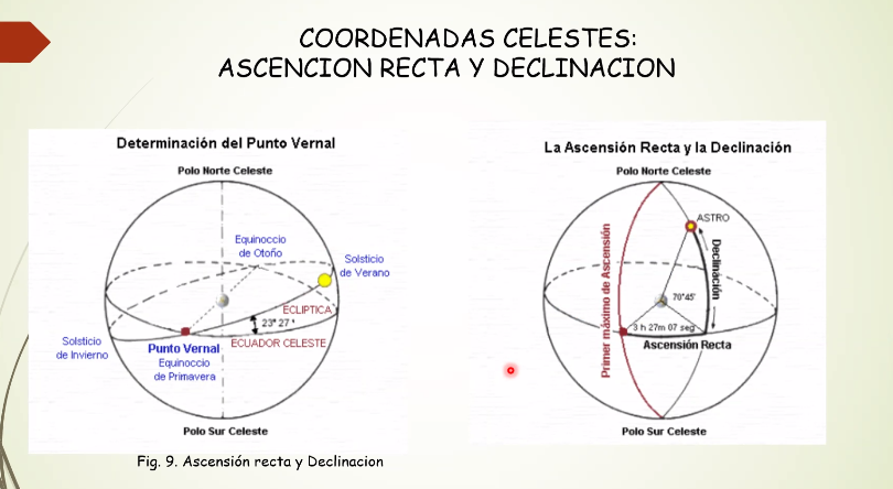
Equatorial Coordinate System: Unlike horizontal coordinate system, this system is independent of the observer’s position and time. It's the most commonly used system for most astronomical applications. This is based on the projection of Earth's equator and rotation axis out into space. The coordinate consists of where RA stands for the right ascension, it starts on in the Vernal Equinox, in the East, we interpolate the rest counterclockwise. So, RA is the projection the lines of longitude onto the celestial sphere. Dec is projection of lines of latitude onto the celestial sphere which starts on in the equator and in the North. Ra is measured in sidereal hours, minutes and seconds, Dec is measured on "degree–minute–second” angle system.
Galactic Coordinate System: This is specific to our galaxy, the Milky Way. The primary coordinates are galactic longitude (l) and galactic latitude (b). This system is useful for studying the structure and movement within our galaxy.
Super-Galactic Coordinate System: This is used to map the large-scale distribution of galaxies in the nearby universe. It centers on the plane of the local super-cluster, a large structure of galaxies that includes the Milky Way.
These coordinate systems allow astronomers to specify an object's position in the sky accurately and communicate those positions to other astronomers consistently.
Telescopes
A telescope is a sophisticated optical instrument designed to capture and magnify light, allowing users to observe distant objects in greater detail. Telescopes play a crucial role in astronomy, aiding astronomers in studying celestial bodies like stars, planets, and galaxies.
Types of Telescopes:
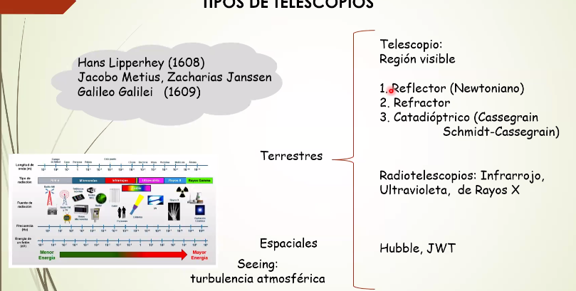
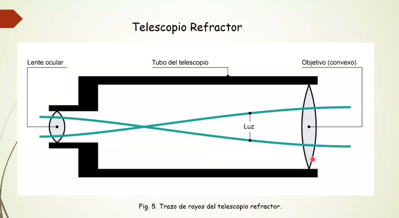
- Refracting Telescopes (Refractors):
- These telescopes use convex lenses to gather and focus light. The primary lens, known as the objective lens, bends (or refracts) light to a focus. Refracting telescopes typically offer sharp images but can be heavy and expensive for their size.
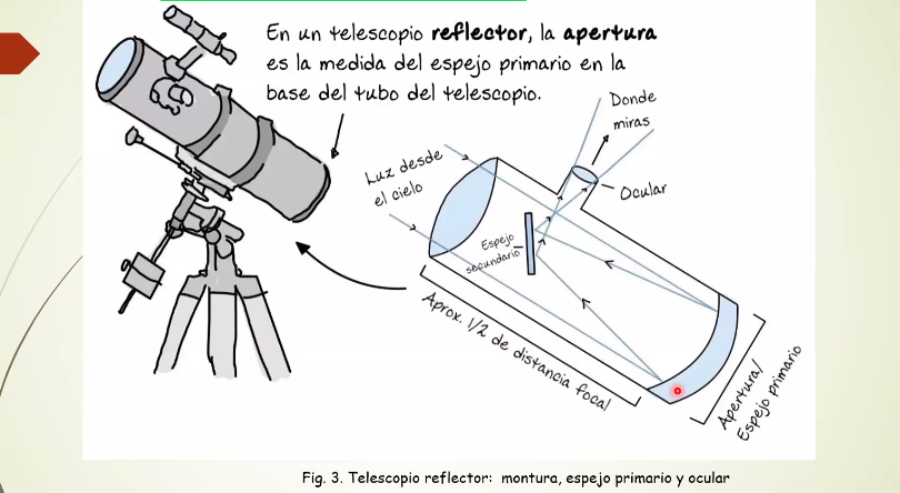
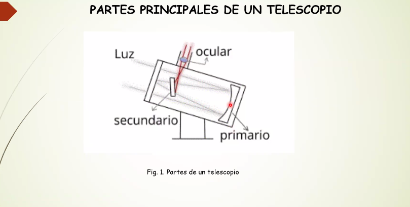
- Reflecting Telescopes (Reflectors):
- Reflectors use a primary mirror to collect and focus light. The light is reflected to a secondary mirror and then through an eyepiece. Reflecting telescopes minimize chromatic aberration and can be more cost-effective for larger apertures.
- Catadioptric Telescopes (Compound Telescopes):
- These telescopes combine lenses and mirrors to gather and focus light. Catadioptric telescopes offer the benefits of both refractors and reflectors, providing sharp images with minimal aberration.
Parts of a Telescope:
Aperture:
- The aperture is the diameter of the telescope's primary lens or mirror. It determines how much light the telescope can gather, affecting its ability to observe faint objects.
Eyepiece:
- The eyepiece is a lens or set of lenses through which the observer views the image. Eyepieces come in various magnifications, allowing the user to zoom in or out on an object.
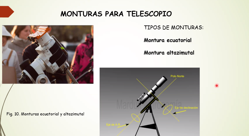
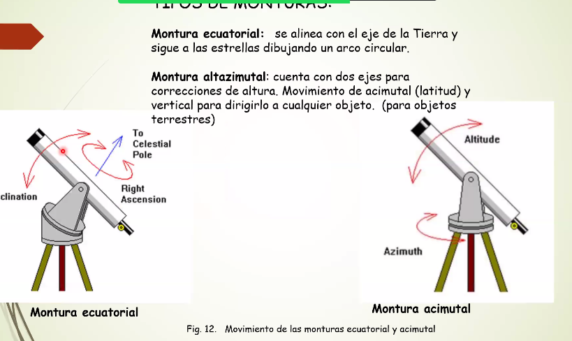
Mount:
- The mount supports the telescope and allows it to pivot. Mounts can be altazimuth (moves up, down, left, and right) or equatorial (compensates for Earth's rotation).
Finder Scope:
- A smaller, low-power telescope mounted on the main telescope to help users locate objects more easily.
Focus Mechanism:
- This mechanism adjusts the focus of the telescope, bringing objects into sharp view.
Tube:
- The tube houses the telescope’s optics. It can be made from various materials, including metal, plastic, or carbon fiber.
Camera:
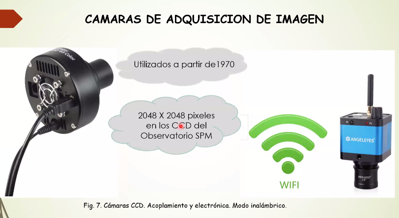
Cameras equipped in telescopes are crucial for capturing and documenting observations. The most common type of camera used in telescopes is an astronomical or astro-camera. Below, you’ll find details regarding the components, types, and uses of cameras within telescopes.
- Sensor:
- The sensor is the component that captures light. The two main types of sensors are Charge-Coupled Device (CCD) sensors and Complementary Metal-Oxide-Semiconductor (CMOS) sensors. CCD sensors are often preferred for their high sensitivity and low noise, while CMOS sensors are faster and more power-efficient.
- Filter Wheel:
- A filter wheel allows the camera to use different filters to isolate specific wavelengths of light, which is crucial for capturing high-contrast images and conducting various types of astronomical research.
- Cooling System:
- Many astro-cameras come with cooling systems to reduce the sensor's temperature, minimizing thermal noise and thereby improving image quality.
- Housing:
- The camera's housing is designed to protect the delicate internal components from the external environment, usually made from materials that minimize thermal expansion and contraction.
Types of Telescope Cameras:
- DSLR Cameras:
- Digital Single-Lens Reflex cameras are popular among amateur astronomers due to their versatility. They can be attached to a telescope using a T-ring adapter.
- Dedicated Astronomy Cameras:
- These cameras are specifically designed for astrophotography. They usually lack a viewfinder, screen, or internal power supply, capturing images that can be viewed and processed on a computer.
- Planetary Cameras:
- As the name suggests, these cameras are optimized for capturing images of planets. They typically have high frame rates to record videos, which can then be stacked to produce still images.
- Solar Cameras:
- These are specialized cameras designed for observing the sun. They often have features that enhance the visibility of solar phenomena, like solar flares and sunspots.
- Webcams:
- Modified webcams can serve as inexpensive options for capturing planetary and lunar images.
Uses:
- Astrophotography:
- Cameras in telescopes are most commonly used for astrophotography, capturing stunning images of celestial bodies like planets, galaxies, nebulae, and stars.
- Scientific Research:
- Professional astronomers use cameras to collect data on various celestial objects and phenomena. These cameras help in measuring light intensity, spectrum, polarization, and other properties essential for astronomical research.
- Monitoring and Surveillance:
- In some cases, cameras are used to monitor the sky continuously for various purposes, like searching for near-Earth objects, monitoring variable stars, or observing transient phenomena like supernovae and meteor showers.
How to Use:
- Attachment:
- Cameras can be attached to telescopes either at the prime focus (replacing the eyepiece) or at the eyepiece itself.
- Focusing:
- Achieving sharp focus is crucial, often done using live view modes or focusing aids provided by camera software.
- Settings Adjustment:
- Depending on the object of interest, users might need to adjust exposure time, ISO sensitivity, and aperture (if applicable).
- Image Capture:
- Images can be captured as single shots, videos, or sequences of exposures.
- Post-Processing:
- Captured images often require post-processing to enhance details, reduce noise, and improve contrast and color balance.
Software
Telescope software plays a vital role in controlling and optimizing the performance of telescopes, especially in astrophotography and astronomical research. This software aids in the telescope's alignment, tracking, focusing, and image capturing processes, providing an easier and more efficient observing experience.
Types of Telescope Software:
- Telescope Control Software:
- This software helps users in managing and controlling their telescope's movement, alignment, and tracking. Telescope control software often supports various telescope mounts and is compatible with a wide range of telescope models.
SharpCap is an astronomy camera capture software primarily designed for astrophotography. SharpCap supports a wide range of astronomy cameras, including those from major manufacturers such as ZWO, QHY, and Altair, as well as standard webcams and USB frame grabbers. It also offers features like plate-solving (which helps to align telescopes accurately), live stacking (which allows users to see a long-exposure view of the sky in real time), and polar alignment correction.
- Planetarium Software:
- Planetarium software provides a visual representation of the night sky, helping users to identify stars, planets, and other celestial objects. It also assists in planning observation sessions by showing what objects will be visible at specific times and locations. Examples are Stellarium and Skyview.
- Astrophotography Software:
- Astrophotography software supports the capturing, stacking, and processing of astronomical images. It helps users to control their camera settings, take a sequence of exposures, and process the captured images to enhance their quality and details.
- Image Stacking Software:
- Image stacking is a technique used in astrophotography to improve the signal-to-noise ratio of captured images. Image stacking software combines multiple exposures to create a single image with reduced noise and enhanced details.
- Focusing Software:
- Focusing software aids users in achieving sharp focus on their target object. It often provides tools and features that simplify the focusing process, like focus aids and autofocus routines.
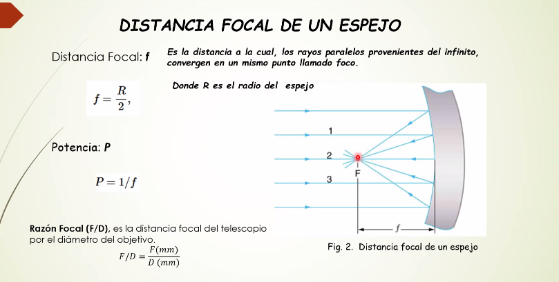
Telescope Mirrors:
- Primary Mirror:
- The primary mirror is the principal light-collecting surface in reflecting and catadioptric telescopes. It gathers incoming light and reflects it toward a focus point.
- Secondary Mirror:
- In some reflecting and all catadioptric telescopes, the secondary mirror redirects the light path to a more convenient viewing location.
Mirrors in telescopes are often coated with a reflective substance, like aluminum or silver, to increase their reflectivity. The quality of the mirrors, their coatings, and their curvature all influence the telescope's performance.
Time series
Viewing a time series as a stochastic process provides a framework to incorporate uncertainty and randomness, and to apply probabilistic and statistical tools for analysis and forecasting.
A stochastic process is a sequence of random variables, indexed by a set. When this set represents time, the stochastic process is referred to as a time series. This type is typical for many time series in econometrics and finance. Conversely, when the index set is continuous (e.g., the set of real numbers), the stochastic process is termed a continuous-time stochastic process, exemplified by phenomena such as Brownian motion. Formally, a stochastic process is a set of random variables where each of them is a real-valued random variable, and belongs to an index set . In this thesis, the term "stochastic process" refers to a piece of information—such as stock prices, inflation rates, etc.—that is assumed to be a discrete-time series. We employ autoregressive models to explain these time series which is a recurrence relation where the current value depends on steps into the past, and some noise , that is, a recurrence of order that has the form for , where is a function that involves consecutive elements of the sequence, for that we need initial values. Also, we will work with multivariate time series where at each time , there are multiple observations. It is an extension of univariate time series data, which consists of single observations recorded sequentially over equal time increments. With multivariate time series data, each time you record data, you record multiple features.
In the following subsections, we will describe some models that serve to address time series forecasting in stock markets in various ways. Each of these models offers a unique approach to time series analysis, with some (like RNN and N-BEATS) stemming from deep learning and others (like ARIMA, ARCH and GARCH) grounded in classical econometrics. The choice of model often depends on the nature of the data, the presence of volatility clusters, and the need for interpretability.
ARIMA
ARIMA, which stands for AutoRegressive Integrated Moving Average, is a class of models that explains a given time series based on its own past values, that is, its own lags and the lagged forecast errors. The general form of an ARIMA model can be expressed as :
where is the order of the autoregressive (AR) model (number of time lags), is the degree of differencing (the number of times the data have had past values subtracted), is the order of the moving average (MA) model, are the parameters of the AR part, are the parameters of the MA part, is the lag operator, represents the time series, and is the error term at time . The AR (autoregressive) part represents the autoregressive part of the model, which uses past values of the series as predictors, the I (Integrated) part represents the order of differencing applied to the time series to make it stationary (constant mean and variance over time), and MA (Moving Average) part accounts for the moving average component, modeling the error term as a linear combination of past error terms.
ARCH
ARCH (Autoregressive Conditional Heteroskedasticity) models capture volatility clustering in financial time series data. It models the variance of the current error term or innovation as a function of the actual sizes of the previous time periods' error terms.
An extension of the ARCH model, GARCH (Generalized Autoregressive Conditional Heteroskedasticity) includes lagged values of both the series' variance and the squared observation. It can model changing variances over time and is especially useful for financial time series where volatility clustering is common.
RNN
A RNN is designed to recognize patterns in sequences of data, such as time series or natural language. It contains loops that allow information to persist and be passed from one step in the sequence to the next. RNNs can be used for various sequence tasks, including time series forecasting. However, traditional RNNs suffer from the vanishing gradient problem, which can make them challenging to train on long sequences. Variants like LSTM (Long Short-Term Memory) and GRU (Gated Recurrent Unit) address this issue.
N-BEATS
N-BEATS (Neural Basis Expansion Analysis) is a recent and interpretable time series forecasting model based on neural networks. It decomposes the input series using basis expansion and then feeds it into a stack of fully connected feed-forward neural networks.
Classification
Single recurrence plot
Methodology
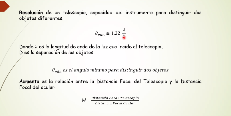
TNOs and other small objects are detected through stellar occultations, which is a cost-effective method for identification. During these occultations, transient flux variations are captured along a chord, resulting in a light curve. We propose employing deep learning to predict features of the observed object using these light curves. The features of the occultation include object diameter , Earth-object distance (in astronomical units) , time offset , angle from opposition , impact parameter , stellar classification , and the readout cadence . However, the parameters of the object —, , — remain unknown.
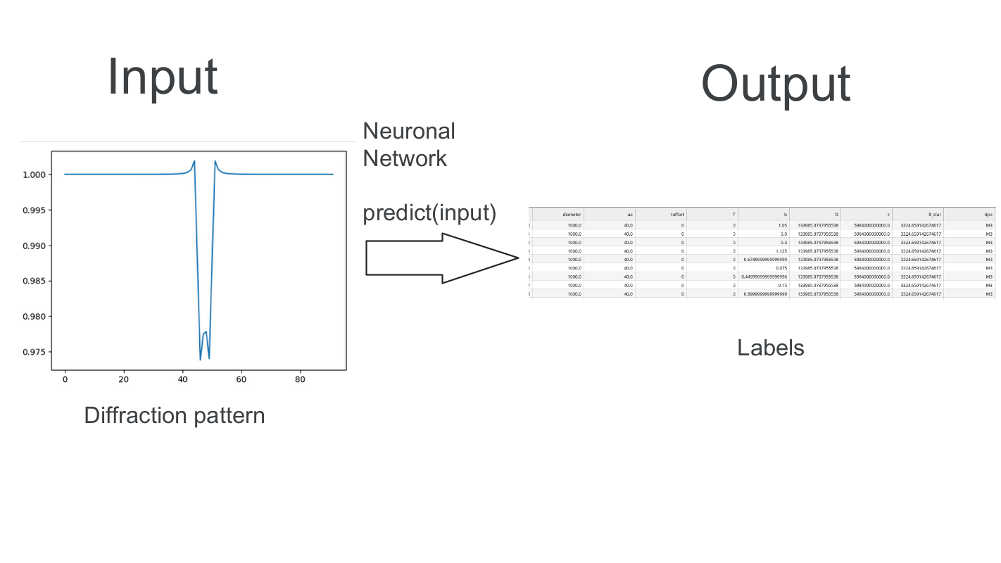
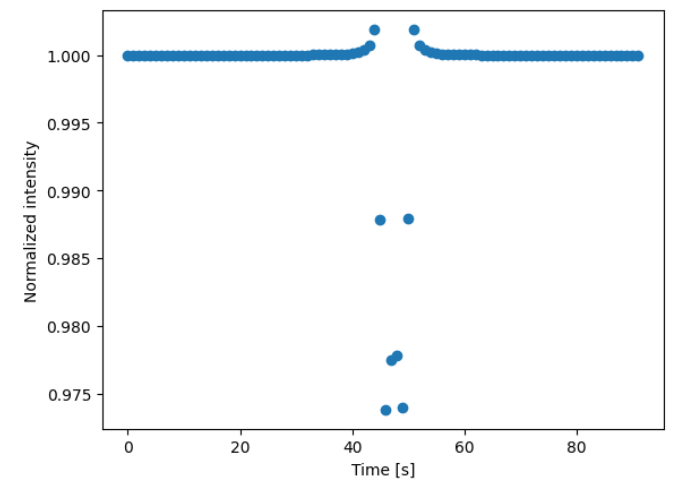
A light curve, also known as a diffraction pattern or diffraction shape, refers to the pattern formed when light interacts with a structure featuring elements on the scale of the light's wavelength. This interaction causes the light to bend, spread, and interfere, creating a characteristic pattern of intensity versus position or angle. Formally, a light curve is a time series, denoted as , consisting of normalized flux values indexed in seconds. Naturally, the diffraction profile with noise must be equal to the light curve .
Generating synthetic light curves
Architecture
The task at hand consists of three activities: remove noise, detect the object at diffraction pattern (anomaly detection) and classify the object.
Detection
Create a simulation dataset
Preprocessing
Train a Sequential GAN with the simulated in order to compress the timeseries3
Predict
Given a timeseries and its decoded representation
Segment the timeseries by applying an "and" filter
Apply a OPTICS algorithm to cluster anomolies
Feature prediction
Classif+ication
Encoding
Results
Conclusions
References
"Astrophysical Techniques" by C.R. Kitchin
Peter Duffett-Smith (1988). Practical Astronomy with Your Calculator, third edition. Cambridge University Press. ISBN 0-521-35699-7.
https://www.sciencedirect.com/topics/earth-and-planetary-sciences/light-curve
https://arxiv.org/pdf/2011.14135.pdf
https://norma.ncirl.ie/5726/1/jonathanflanagan.pdf
Occultations by Small Non-spherical Trans-Neptunian Objects. I. A New Event Simulator for TAOS II in https://iopscience.iop.org/article/10.1088/1538-3873/ab152e
The TAOS II Survey: Real-time Detection and Characterization of Occultation Events in https://iopscience.iop.org/article/10.1088/1538-3873/abd4bc
Pattern Recognition Using SVM for the Classification of the Size and Distance of Trans-Neptunian Objects Detected by Serendipitous Stellar Occultations in
https://dx.doi.org/10.1088/1538-3873/ac7f5c
Hernández-Valencia, B., Castro-Chacón, J., Reyes-Ruiz, M., Lehner, M., Guerrero, C., Silva, J., Hernández-Águila, J., Alvarez-Santana, F., Sánchez, E., Nuñez, J., Calvario-Velásquez, L., Figueroa, L., Huang, C., Wang, S., Alcock, C., Chen, W., Granados Contreras, A., Geary, J., Cook, K., Kavelaars, J., Norton, T., Szentgyorgyi, A., Yen, W., Zhang, Z., & Olague, G.
(2022). Pattern Recognition Using SVM for the Classification of the Size and Distance of Trans-Neptunian Objects Detected by Serendipitous Stellar Occultations.
Publications of the Astronomical Society of the Pacific, 134(1038), 15
https://www.youtube.com/watch?v=2K3ScZp1dXQ
https://www.youtube.com/watch?v=n9WaLsyVjUQ
Diffraction calculation of occultation light curves in the presence of an isothermal atmosphere.
Appendices
Management
Deployment
Desktop app to web app
This project allows you to transform desktop apps into web apps. After you set up your operating system, Dockerfile.
https://github.com/sanchezcarlosjr/desktop-app-to-webapp/
Occulation detector
https://github.com/sanchezcarlosjr/occultation_detector
https://github.com/sanchezcarlosjr/taos_ii_neuronal_networks
Web app (App virtualization)
Software Architecture
classDiagram
    class Simulator
    class ObservationParemeters
    class Prediction {
       calculate_parameters()
    }
    class Model
Diagram sequence
sequenceDiagram
    User->>+Simulator: run with parameters
    Simulator->>Simulate["Arrokth"]: run with parameters
Reporte
FITS and SExtractor
https://astrometry.net/use.html
https://sextractor.readthedocs.io/en/latest/Introduction.html