
Scientific Computing
Prerequisites
- Single variable calculus.
- Linear algebra.
- Algorithms
Introduction
Approximation of Real number to some procession.
Pay for precision with time.
Resources
Resources
Key questions
Numerical analysis, numerical methods, or symbolic calculation
Differences
| Name | Differences | Similarities |
|---|---|---|
| Numerical analysis | ProofRigorousnumerical methods | Algorithms |
| Numerical methods | Algorithms | |
| Symbolic calculation | Deductive |
Octave, Matlab, Mathematica, Maxima, Python, or Julia
Story
William Kahan
[1] https://archive.siam.org/meetings/la09/talks/benzi.pdf
https://mathshistory.st-andrews.ac.uk/Biographies/Seidel/
Octave
Glosario
Modelo matemático. Descripción de un sistema (fenómeno, procedimiento, procedimiento …) usando la teoría (gramatica, principios, sus reglas) de alguna de las áreas de las matemáticas (análisis numérico, ecuaciones diferenciales, teoría de automatas, probabilidades, topología, …) .
Exactitud. Cualidad de conocimiento sobre la magnitud real.
Precision. Dispersión del conjunto de valores obtenidos o medidos de un instrumento.
Sesgo o inexacitud. Diferencia entre la magnitud real y los valores obtenidos.
Incertidumbre o imprecision. Dispersión tendiendo a cero de los valores obtenidos de un instrumento.
Accuracy and precision
Bias.
ISO 5725-1 ISO/DIS 5725-1
Mathematical preliminaries and Error Analysis
1.1 Review of Calculus
Worked examples
- Show that the following equations have at least one solution in the given intervals.
As is continuous and
,
The Intermediate Value Theorem implies that a number x exists, with .
If and 0 is a number between and , then there exists a number in for which .
- Find intervals containing solutions to the following equations.
1.2 Round-off Errors and Computer arithmetic
Def. Floor function
Def. Chopping or truncating is a function such that
Def. Suppose that is an approximation to .
Ceil and floor
https://stackoverflow.com/questions/6208488/implementation-of-ceil-and-floor
Cast
https://stackoverflow.com/questions/22330575/how-are-typecasts-in-c-implemented
https://en.wikipedia.org/wiki/Loop_unrolling
How Many Decimals Do We Really Need?
Floating-Point Computation by Pat Sterbenz
- IEEE 754
How calculating more precise than double or long double? How to increase precision by hundreds of decimals?
Use C++, and then use https://gmplib.org/#DOWNLOAD, other languages https://en.wikipedia.org/wiki/GNU_Multiple_Precision_Arithmetic_Library
Leijen, Daan (December 3, 2001). "Division and Modulus for Computer Scientists" (PDF). Retrieved 2014-12-25.
How can minimize the error upon arithmetic operations?
- Minimize the number of arithmetic calculations.
- Polynomials should always be expressed in the nested form before performing an evaluation.
- Use rounding over chopping.
- Prioritize the operations by error-producing sum, multiplication, and division.
Worked examples
- Determine the six-digit a) chopping and b) rounding values of the .
Chapter notes
https://www.youtube.com/watch?v=JTinepDn1dI&ab_channel=OscarVeliz
Solutions of Equations in One Variable
Is there any way to find the number of real roots of a polynomial computationally?
Bisection method
Fixed-point iteration
Newton-Rapshon method
Summary
Worked examples
- Da la definicion de numero de maquina en la forma de punto flotante decimal normalizado.
Sea el punto flotante decimal normalizado analogo al punto flotante binario normalizado para representar las operaciones de los numeros de maquina segun el IEEE754 en base 10 y siendo inspirado en la normalizacion de la notacion cientifica (aqui tomamos ), a saber, el punto flotante decimal normalizado tiene la forma:
donde es distinto de 0 () y los siguientes terminos del significando o mantisa son cualquier numero menor a la base 10 (), 10 es nuestra base , el expontente y digitos decimales del numero de maquina tal que
Ejemplo:
porque
2.a
Si ,
entonces por regla de L’Hopital (*)
Si ,
entonces por *
2. b
Redondeo a 4 digitos.
2.c
- d
2.e
- Usa el metodo de Steffensen para encontrar una aproximacion a la raiz de
con , y usa al menos 10 digitos en los calculos.
Vas a poner las formulas o ecuaciones que usaste en cada uno de los calculos aritmeticos que realizaste.
- Find root of a number using Newton’s method
https://opensource.apple.com/source/Libm/Libm-47.1/ppc.subproj/sqrt.c.auto.html
https://math.mit.edu/~stevenj/18.335/newton-sqrt.pdf
https://math.stackexchange.com/questions/296102/fastest-square-root-algorithm
https://stackoverflow.com/questions/63450864/ieee-754-conformant-sqrt-implementation-for-double-type
Tabla comparativa
| Metodo | Diferencias | Ventajas | Desventajas |
| Biseccion | Basado en el teorema del valor intermedio, determinando cualquier intervalo lo satisface hasta lograr la tolerancia deseada. Por tanto, necesita un intervalo [a,b]. | El mas simple de implementar. No necesita calculo de derivada. Siempre converge a la raiz. | El mas lento por su radio de convergencia. No encuentra raices complejas. Buenas aproximaciones pueden ser rechazadas. |
| Netwon-Rapshon | Metodo de punto fijo, que necesita del calculo de la derivada. Necesitando un punto como entrada. siempre que M= | El mas rapido, su radio de convergencia es | Necesita calculo previo de derivada. No encuentra raices complejas. el metodo diverge. Depende en gran medida de para converger (no esta en el intervalo) |
| Secante | Metodo de punto fijo, que NO necesita del calculo de la derivada, usando su aproximacion mediante la def. Necesitando dos puntos de la secante como entrada. | No necesita calculo de derivada. | No encuentra raices complejas. Puede diverger. |
| Regula falsi | Adaptacion del metodo de la secante y biseccion que asegura que la raiz este en el intervalo . | No necesita calculo de derivada. | No encuentra raices complejas. No es recomendado por (Burden, 73). |
| Müller | Basado en metodo de la secante, pero en vez de una linea usamos una parabola, por tanto, necesitamos 3 puntos. . | No necesita calculo de derivada. Calcula raices complejas. | Puede diverger. |
| Halley | |||
| Householder-n |
http://www.math.usm.edu/lambers/mat460/fall09/lecture7.pdf
https://math.stackexchange.com/questions/2473794/asymptotic-order-versus-order-of-convergence
Interpolation
https://gist.github.com/sanchezcarlosjr/6cd5f027740e964c4a45cb0880dc18ae
https://gist.github.com/sanchezcarlosjr/74ab156989087338a6d27227817a7a22
Kochanek–Bartels spline
Bezier curves
https://docs.scipy.org/doc/scipy/tutorial/interpolate.html
Numerical linear algebra
Solving Linear Systems
https://gist.github.com/sanchezcarlosjr/9edad3c66853ca24de3e97104cf68261
Gauss-Jordan
LU factorization
Approximate solutions by iterations
Exact solutions tend to be inefficiency . Our computers save us by their power processing in complex calculations. Thus the methods were born.
We say that a method approximate to the solution from an arbitrary initial vector where each k iteration tend to such that .
The method converges when , otherwise it diverges.
Jacobi method
This method was discovered by Carl Gustav Jacob Jacobi, which use triangular matrices.
https://sci-hub.do/https://doi.org/10.1080/0020739980290204
https://arxiv.org/pdf/1304.2097.pdf
https://www.coe.pku.edu.cn/attachments/dc028aad92c84efdafe6b9f65f1f0d48.pdf
https://core.ac.uk/download/pdf/82202439.pdf
Seidel method
This method was discovered by Philipp Ludwig von Seidel. We now (inappropriately) call the Gauss-Seidel method [1], which improves the Jacobi method. Honor to whom honor is due.
Methods of Conjugate Gradients
SVD
https://cims.nyu.edu/~donev/Teaching/NMI-Fall2014/Lecture5.handout.pdf
Elementary function computations
For computations with very high precision, the algorithms based on the elliptic integrals are among the fastest known today for the logarithm, the number π, and the exponential function.
Logarithms, pow, gamma,
Notes
https://www.jjj.de/fxt/fxtbook.pdf
Numerical differential equations
https://gist.github.com/sanchezcarlosjr/80aa8c039d71bea3decc86fb744f719f
Los métodos más comunes para resolver este tipo de problemas incluyen el método de las diferencias finitas, el método de los elementos finitos, y el método de Runge-Kutta.
Numerical analysis, numerical methods, or symbolic calculation
Random number generation
Log
- Count the number of digits
By mod. Its time complexity is
def algorithmMod(n):
  count=0
  while(n>0):
    count=count+1
    n=n//10
  return count
By log. Its time complexity is
def algorithmLog(number):
  return math.floor(math.log10(math.abs(number)))+1
https://replit.com/join/zpwivezz-carlossanchez14
Modulo operation
Remainder after division.
Worked examples
- Extracting individual digits.
Truncate
Floor and ceil
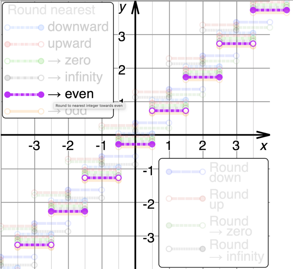
Rounding
Round half to even, a variant of the round-to-nearest method.
This method is called the round-to-even method. Other names include the round-half-to-even method, the round-ties-to-even method, and "bankers' rounding." This variant of the round-to-nearest method is also called convergent rounding, statistician's rounding, Dutch rounding, Gaussian rounding, odd–even rounding, or bankers' rounding.
Banker's rounding: the value is rounded to the nearest even number. Also known as "Gaussian rounding", and, in German, "mathematische Rundung".
Standard rounding: the value is rounded to the nearest number (be it odd or even). In German it is known as "kaufmännische Rundung".

754-2019 - IEEE Standard for Floating-Point Arithmetic since 1985.
https://en.wikipedia.org/wiki/Rounding
If the fractional part of x is 0.5, then y is the even integer nearest to x.
 https://jsfiddle.net/2hs9nqbk/2/
function roundIt(n, d = 0) {
            var m = Math.pow(10, d);
            var n = +(d ? n * m : n).toFixed(8);
            var i = Math.floor(n),
                diff = n - i; // getting the difference
            var e = 1e-8; // Rounding errors in var(diff)
            // Checking if the difference is less than or
            // greater than, based on that adding the 1 to it.
            var r = (diff > 0.5 - e && diff < 0.5 + e) ?
                ((i % 2 == 0) ? i : i + 1) : Math.round(n);
            return d ? r / m : r; // if d != 0 then returning r/m else r
}
https://www.geeksforgeeks.org/gaussian-bankers-rounding-in-javascript/
Experimental
import time
import numpy as np

def timer(f):
  x=np.random.rand(1,100000)[0]
  times = []
  for i in range(10):
    tic = time.perf_counter()
    f(x)
    toc = time.perf_counter()
    times.append(toc - tic)
  print(f"Build finished in {np.mean(times):0.4f} +- {np.std(times):0.4f} seconds")
Seminumerical Algorithms. Arithmetic.
Numerical analysis.
Matrix operations.
The Fast Fourier Transform
Integer and Polynomial Arithmetic
Number-Theoretic Algorithms
References
Burden, R. L. y Faires, J. D. (2015). Análisis numérico. (9a ed.).
Cengage Learning.
Chapra, S. C. (2017). Applied numerical methods with MATLAB for engineers and scientists. (4a ed.). Mcgraw-Hill Education.
Demanet, L., (2012). Introduction to numerical analysis. MIT
opencourseware.
https://ocw.mit.edu/courses/mathematics/18-330introduction-to-numerical-analysis-spring-2012/
Epperson, J. F., (2021). An introduction to numerical methods and analysis. (3a ed). Wiley.
Gezerlis, A., (2020). Numerical methods in physics with python. Cambridge University Press.
Howard II, J. P., (2020). Computational methods for numerical analysis with R. CRC Press
Fausett, L.V. (2002). Numerical methods: algorithms and applications. Pearson.
Gerald, C.F. y Wheatley, P.O. (2001). Análisis numérico con aplicaciones (6a ed.). Prentice Hall.
Stoer, J. & Bulirsch, R. (1993). Introduction to numerical analysis.Springer-Verlag.