K-Means and association rules in Weka
K-Means
We analyze agricultural datasets from New Zealand with K-Means (https://www.cs.waikato.ac.nz/~ml/weka/agridatasets.jar), in particular, we will group the eucalyptus dataset.
% Attribute Information:
% 1. Abbrev - site abbreviation - enumerated
% 2. Rep - site rep - integer
% 3. Locality - site locality in the North Island - enumerated
% 4. Map_Ref - map location in the North Island - enumerated
% 5. Latitude - latitude approximation - enumerated
% 6. Altitude - altitude approximation - integer
% 7. Rainfall - rainfall (mm pa) - integer
% 8. Frosts - frosts (deg. c) - integer
% 9. Year - year of planting - integer
% 10. Sp - species code - enumerated
% 11. PMCno - seedlot number - integer
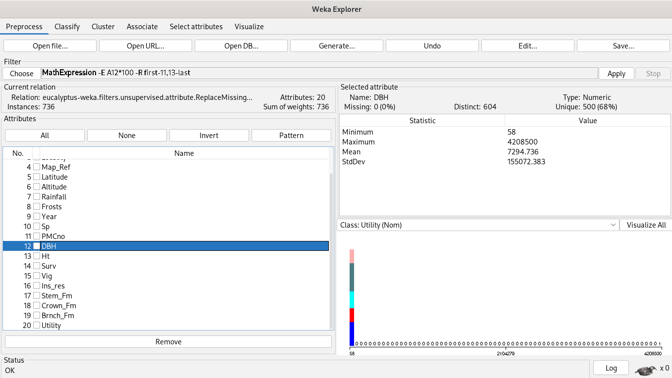
% 12. DBH - best diameter base height (cm) - real
% 13. Ht - height (m) - real
% 14. Surv - survival - integer
% 15. Vig - vigour - real
% 16. Ins_res - insect resistance - real
% 17. Stem_Fm - stem form - real
% 18. Crown_Fm - crown form - real
% 19. Brnch_Fm - branch form - realSince K-Means’ input are continuous features, our analysis starts by choosing the best diameter base height (DBH) and height (Ht) features. However, they have different units and missing values first, we’ll apply the filter “remove missing values”, “a mathematical expression” and “normalization” in order to keep away bad results.
Analysis
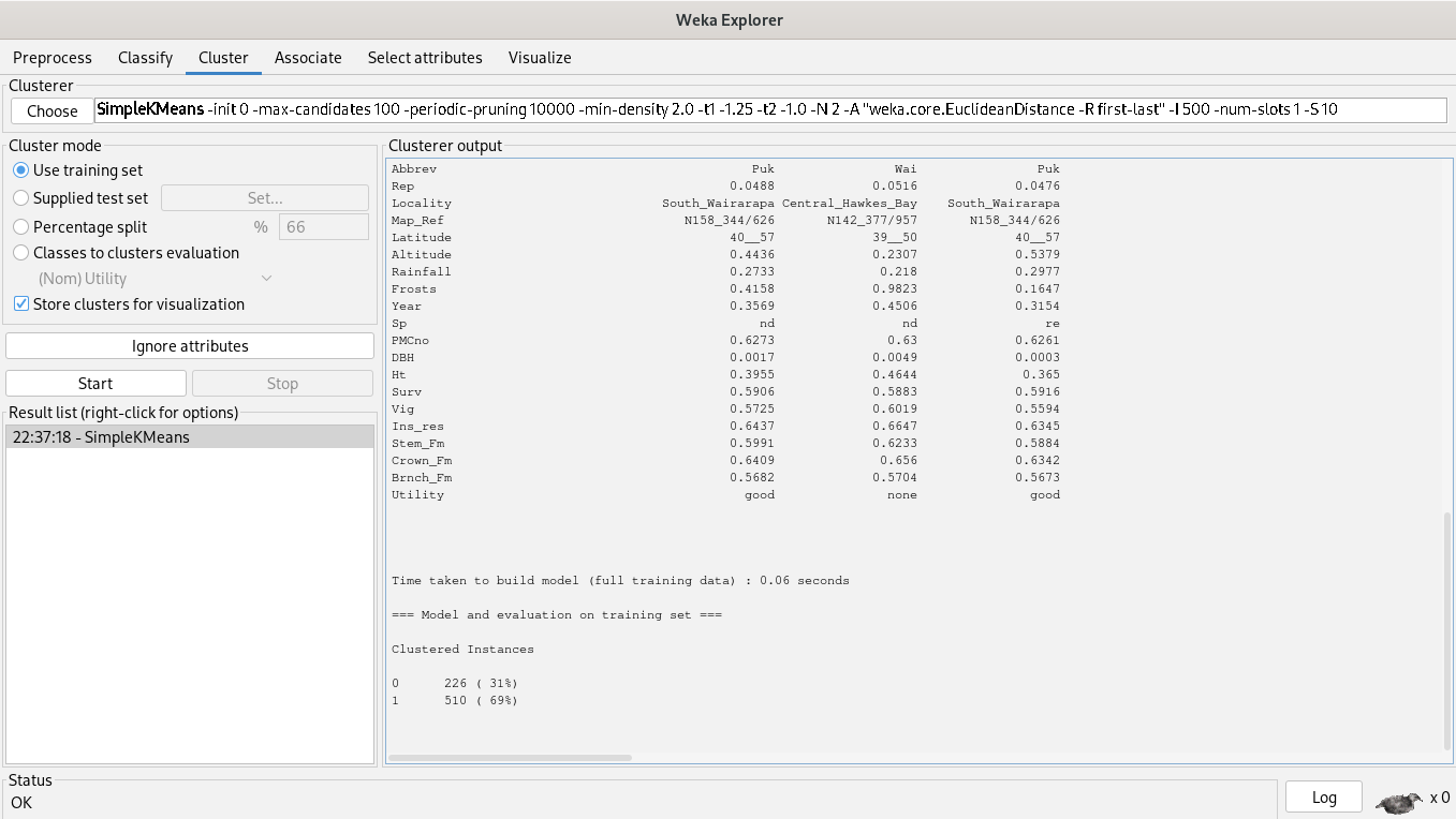
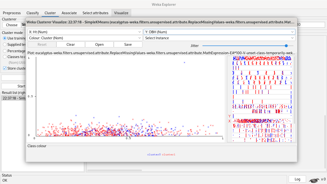
69% of clustered instances belong to cluster 1 and 31% of clustered instances belong to cluster 0, but our plot said another thing, instances are really close, so, a simple K-Means algorithm is unuseful, it doesn’t help to segment instances.
Association rules
We start from zero opening again our dataset.
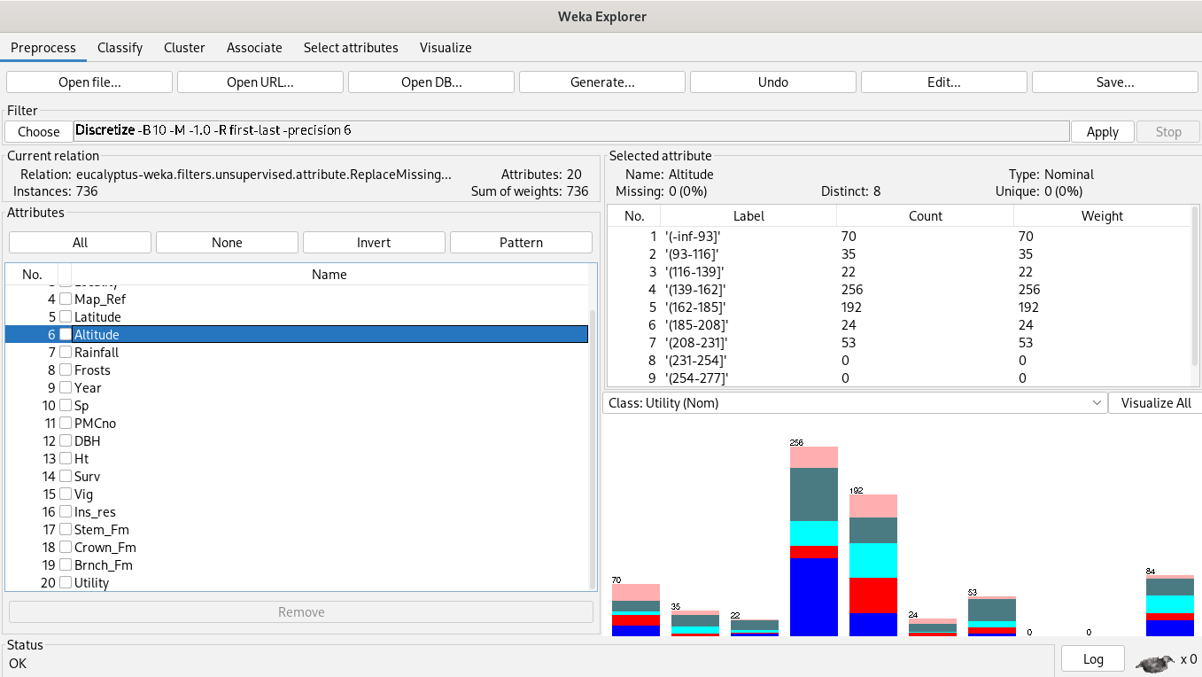
Association rules algorithms’ inputs are categorical variables, so we discretize first.
We’re associating attributes by choosing the Apriori algorithm.
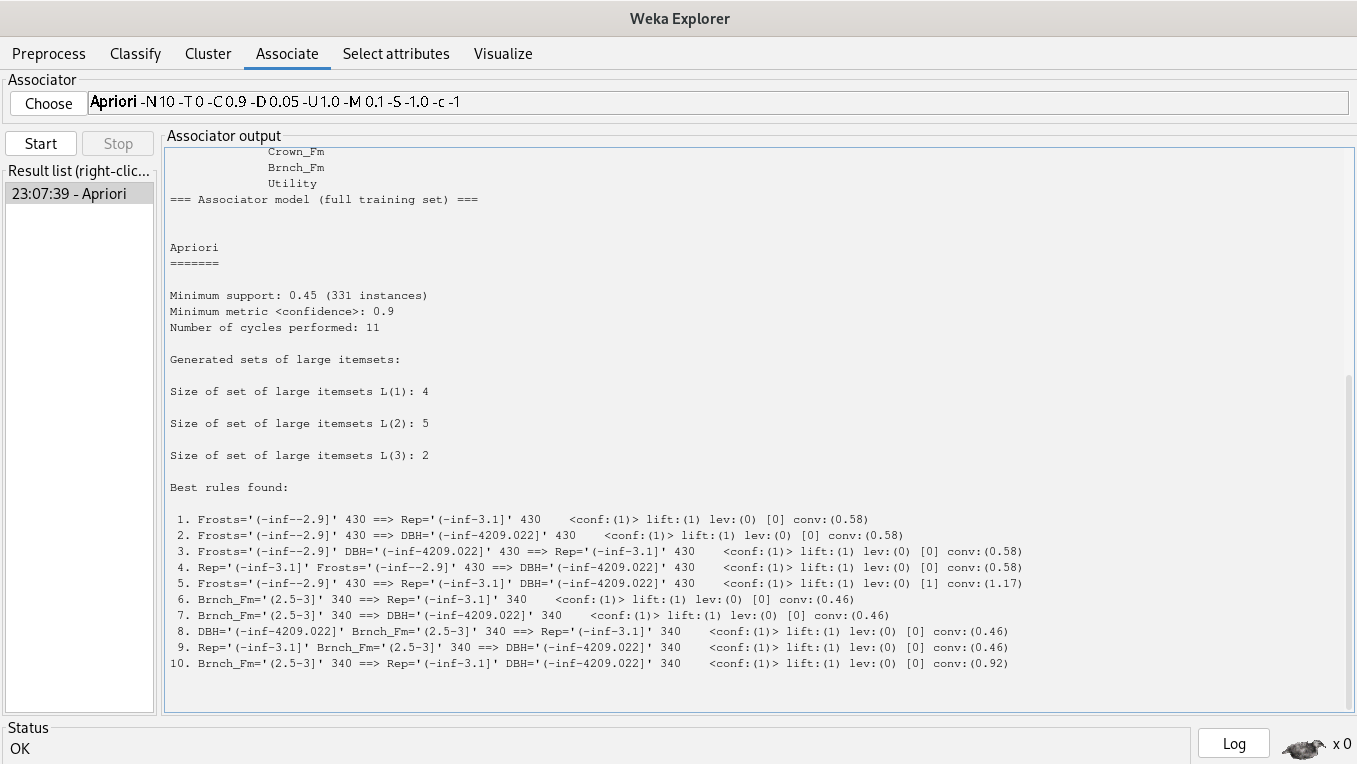
The rules are the following:
1. Frosts='(-inf--2.9]' 430 ==> Rep='(-inf-3.1]' 430    <conf:(1)> lift:(1) lev:(0) [0] conv:(0.58)
2. Frosts='(-inf--2.9]' 430 ==> DBH='(-inf-4209.022]' 430    <conf:(1)> lift:(1) lev:(0) [0] conv:(0.58)
3. Frosts='(-inf--2.9]' DBH='(-inf-4209.022]' 430 ==> Rep='(-inf-3.1]' 430    <conf:(1)> lift:(1) lev:(0) [0] conv:(0.58)
4. Rep='(-inf-3.1]' Frosts='(-inf--2.9]' 430 ==> DBH='(-inf-4209.022]' 430    <conf:(1)> lift:(1) lev:(0) [0] conv:(0.58)
5. Frosts='(-inf--2.9]' 430 ==> Rep='(-inf-3.1]' DBH='(-inf-4209.022]' 430    <conf:(1)> lift:(1) lev:(0) [1] conv:(1.17)
6. Brnch_Fm='(2.5-3]' 340 ==> Rep='(-inf-3.1]' 340    <conf:(1)> lift:(1) lev:(0) [0] conv:(0.46)
7. Brnch_Fm='(2.5-3]' 340 ==> DBH='(-inf-4209.022]' 340    <conf:(1)> lift:(1) lev:(0) [0] conv:(0.46)
8. DBH='(-inf-4209.022]' Brnch_Fm='(2.5-3]' 340 ==> Rep='(-inf-3.1]' 340    <conf:(1)> lift:(1) lev:(0) [0] conv:(0.46)
9. Rep='(-inf-3.1]' Brnch_Fm='(2.5-3]' 340 ==> DBH='(-inf-4209.022]' 340    <conf:(1)> lift:(1) lev:(0) [0] conv:(0.46)
10. Brnch_Fm='(2.5-3]' 340 ==> Rep='(-inf-3.1]' DBH='(-inf-4209.022]' 340    <conf:(1)> lift:(1) lev:(0) [0] conv:(0.92)
Since real datasets have thousands of instances, we are showing you how to calculate association rules metrics.
Suppose you’re developing a recommendation system for a streaming company with authors Itemset={Mozart, Chopin, Handel, Bach, Queen, Chuck Mangione}. You associate them by extracting the association rule
where .
Suppose the following dataset
| Mozart | Handel | Bach | Chopin | Queen | Chuck Mangione | |
| User 1 | X | X | ||||
| User 2 | X | X | X | X | ||
| User 3 | X | |||||
| User 4 | X | |||||
| User 5 | X | X | ||||
| User 6 | X | X | X |
If a person listens Mozart and Handel, then he or she listens to Bach. Other words,
How do we measure this association rule's strengths?
Support.
So,
Confidence.
So,
Lift.
So,